¶ SmartFlow V2
¶ Introduction
Formulating an exact mathematical formula for finding the best charge and discharge plan in different everyday situations is a complex task. SmartFlow V2 is a notable improvement over its predecessor, V1, drawing upon the wisdom and insights gained from prior versions. It places a strong focus on implementing established rules to examine and assess a wide range of possible charging plans. These rules are guided by input factors like past household energy usage, anticipated sunlight availability, electricity rates, and more. Through this approach, it aims to intelligently construct an effective energy management strategy.
¶ Hypothesis
If I knew which hours to use for charging during expensive times, I could maximize my savings.
But here's the catch: if I start by charging the battery at the cheapest hour (let's say hour 1) to have enough power for the most expensive hour (hour 24), I can't use any of the hours in between for charging or discharging. Refer to Appendix 1.

Now, if we assume that each charging hour fills the battery completely and each discharging hour empties it completely, the best scenario would be to increase the number of charge and discharge cycles as long as it's still financially worth it.
A perfectly planned charge schedule might look like Appendix 2.

If we compare Appendix 1 and Appendix 2, with each little square representing 1 euro, we see that Appendix 1 would save 17 euros in total. However, Appendix 2 would save 12 euros between hour 1 and 3, then 4 euros between hour 5 and 8, and finally, 14 euros between hour 12 and 24, adding up to a total of 30 euros. That's 13 euros more than the plan in Appendix 1.
But here's the challenge: when should we charge and discharge the battery? We can't simply rely on the price because it can be both cheap and expensive based on our charge plan.

In Appendix 3, you can see examples on hours 5, 8, 10, and 20 where the same hourly price can be considered either cheap or expensive depending on the surrounding hours.
To tackle this, for each "expensive hour," we maintain a list of available cheap hours. For every expensive hour, we aim to reserve power during the cheapest available hour. The tricky part is figuring out the order in which to reserve power during the expensive hours to avoid blocking a cycle like in Appendix 1.
In Appendix 4, we reveal a superior approach by rearranging the order in which we reserve power during the expensive hours. For example, reserving hour 6 on hour 1, hour 9 on hour 8, and hour 24 on hour 19 leads to entirely different charge plans that result in substantial savings. The remaining expensive hours can't be used for discharging in this specific arrangement.

The real challenge now is figuring out the best order for reserving power during the expensive hours. Instead of relying on complex mathematical formulas, we could try every possible order and calculate the potential savings for each order. This way, we can theoretically always find the best charging plan.
¶ Parameters
¶ Consumption estimation
We project energy consumption for the next 24 hours by considering historical data. We aggregate the consumption for the same hour from the previous days and calculate the average. This average serves as our estimate for that specific hour.
¶ Estimation of own production
This feature is currently compatible only with the KSTAR device, designed for tracking the peak PV power generated by solar panels. It maintains a historical record of peak power for each hour, with a small daily reduction to adapt to seasonal variations.
To estimate the power generation for a specific hour today, we use the historical peak PV power for that same hour. The estimation is calculated using the formula:
(Peak PV power for the specific hour) * (hourly factor) => (estimated kilowatt-hours) * (adjusted for local cloud coverage) = (final estimated kilowatt-hours)
The "cloud coverage" factor considers the current weather conditions in the city where the solar installation is located.
¶ Find all orders of expensive hours (Permutations)
The primary focus of this algorithm lies in the comparison of various charge plans. To initiate this comparison, it's essential to define all available charge plans that require computation.
For every hour, we compile a list of historical electricity prices for that specific hour with the condition that if SmartFlow charged the battery in the historical hour and discharged it in the current hour, it would result in an economic gain per kilowatt-hour exceeding a predefined threshold. We refer to this list as "Legal Hours".

In Appendix 5, you can see an example where each hour now has its own internal list of legal hours. These hours are selected based on a price difference of at least 4 mini squares. In other words, for instance, hour 5 can legally reserve power from hours 1, 2, 3, and 4 and still meet the predefined gain threshold per kilowatt-hour.
Upon completing this process, we can identify the expensive hours, as they have at least one associated Legal Hour. This implies that discharging the battery during these hours would result in an economic gain exceeding the established threshold. Please note that this list is limited to a maximum of 12 "expensive" hours.
After identifying these expensive hours, we can generate all possible order permutations for them. This ensures that each charge plan varies.
It's important to note that an expensive hour can still be reserved for charging in preparation for another hour that might be even more expensive.
¶ Control algorithm
¶ Generate a chargeplan for each permutation
For every possible arrangement of expensive hours, our task is to create a workable charging plan and figure out the potential financial benefit. Each arrangement contains a random order of the specified expensive hours, each with a specific number of suitable legal hours, the hourly electricity cost, and the anticipated home power usage.
- Our charging plan starts with the first expensive hour in the specified sequence, and then move through the hours one by one in that order.
- We first check if the current hour is already set for charging another expensive hour. If it is, we move on to the next expensive hour in line.
- Then we check the list of legal hours, starting with the cheapest and moving up to the most expensive. Our aim is to identify an available hour for charging, provided there's room in the battery. If we find such an hour, we allocate the house's power consumption to it. If the cheapest hour is unavailable, we proceed to the next less expensive option.
- After locating a cost-effective charging hour, we make sure that the last expensive hour designated for discharging matches with this affordable charging hour, and that the price difference between these hours is greater than a set threshold. This check prevents situations where we discharge the battery at a certain price and then recharge it at the same price.
- We then move on to the next expensive hour in the sequence.
- Once we've considered all the expensive hours and assembled a charging plan, we conduct a final check. We examine the chronological order of charge and discharge events, ensuring that each pair maintains a price difference of at least the predetermined threshold. This meticulous check determines whether the charging plan is valid. If this condition is not met, the plan is considered invalid.
- If we have a valid charging plan, we calculate the expected financial gain. If we discover a new plan with the highest potential gain, we save it.
- We'll circle back to point 1 and try the next permutation, reconfigureing the order of the predefined expensive hours.
To handle the vast number of potential arrangements, which can reach up to 24! (24 factorial), we employ a practical strategy. This strategy involves using statistical insights and early terminations for unworkable plans, balancing computational efficiency with the pursuit of the best solution in real-world scenarios.
We closely monitor each iteration, and when we observe no further improvements over a predefined number of plans, we conclude the process. At this point, we return the best charging plan found so far, aiming to maximize efficiency while seeking the most advantageous solution.
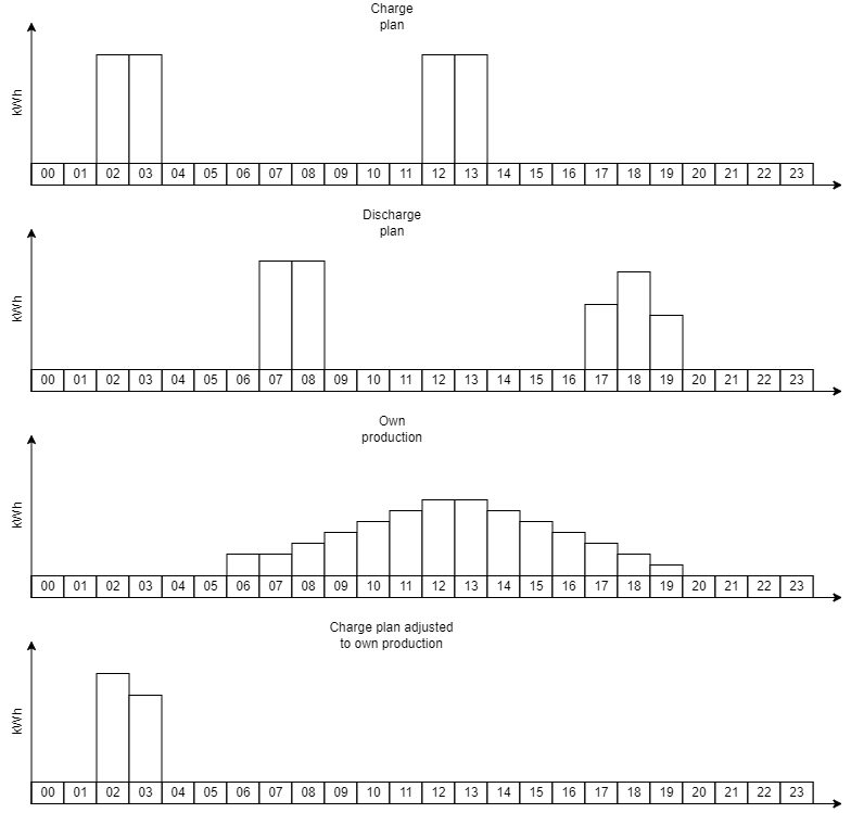
¶ Adjusting charge plan for own production
After a charge and discharge plan has been calculated, the self-production is deducted from the hours where it can be seen that the self-production can be used to charge the battery instead of the grid. It selects the hours with the highest sell price first and then works to the lowest sell price because if exporting its production to the grid it should be done when the sell price is highest.